Harmonics has always been of special concern in power system studies. In the past the power system comprised mainly of passive components with relatively linear operating range and synchronous generators. Harmonic analysis of such systems is the state-of-the art right now.
The wind turbines are nowadays mainly connected together into a collector system through a widespread network of medium voltage (MV) sub-sea cables. The voltage is then stepped up and the wind power plant (WPP) is connected to the power grid through long high voltage (HV) cables which constitute the HVAC or HVDC transmission system. Such configuration is still being challenging to the industry from harmonic generation, propagation and stability perspective [1].
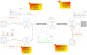
The presence of harmonics inside the WPP is a nuisance as it leads to higher current and voltage levels in the system. Consequently, the system loss is higher system, and there is higher component stress. Moreover, if there is series or parallel resonance points in the WPP, the resonating harmonics may get amplified and then that can be destructive. The resonance can be series or parallel type as shown in Fig. 1. Besides, there are other issues with harmonic interference and power quality [2].
Identification of the presence of harmonics in the system and potential resonance conditions are very critical for the design of a WPP. Measurement of harmonic content is an important element of the WPP and wind turbine evaluation process. Measurement of field data is also required to validate the theoretical analysis and numerical simulations. The measurement equipment should be carefully adjusted in order to record harmonics of interest with acceptable accuracy and precision.
The harmonic measurements should be carried out during continuous wind turbine normal operation, i.e. fault free operation complying with the description in the wind turbine manual excluding wind turbine start-up and shutdown as described in IEC 61400-21. Since different operational modes are characterized by different frequency response of the converter thereby affecting the harmonic emission, the operational modes should be considered, and any change in the mode should be noted during the measurement process [3].
It is also recommended to perform measurements when the wind turbines are not operational such that the harmonic background spectrum can be evaluated. The wind turbine during background measurements should neither inject nor absorb any harmonic current during this process.
Harmonic mitigation by design is affected by several uncertainties in different factors during the design of a WPP. Some of them are listed below:
- Lack of accurate models provided by the manufacturers.
- Component tolerances in the WPP model.
- Wind turbine harmonic emission model uncertainties.
- Phase angle between harmonics from different wind turbines and possible harmonic cancellation.
- Different operating modes of the wind turbines (e.g. power production levels, wake effects, voltage control, etc.).
- Lack of reliable information from TSOs and DSOs for the external network model.
- Changes in the wind turbine converter controller affecting harmonic emission.
- Linear model of WPP components (e.g. transformers, converters, cables, etc.).
- Linear harmonic load flow calculation method excluding possible frequency coupling.
[1] Ł. H. Kocewiak, C. L. Bak, J. Hjerrild, "Wind Turbine Converter Control Interaction with Complex Wind Farm Systems," IET Renewable Power Generation, Vol. 7, No. 4, 2013.
[2] Ł. H. Kocewiak, S. K. Chaudhary, B. Hesselbæk, "Harmonic Mitigation Methods in Large Offshore Wind Power Plants," in Proc. of The 12th International Workshop on Large-Scale Integration of Wind Power into Power Systems as well as Transmission Networks for Offshore Wind Farms, Energynautics GmbH, London, UK, 22-24 October 2013, 443-448.
[3] Ł. H. Kocewiak, "Harmonics in Large Offshore Wind Farms," PhD Thesis, Aalborg University, Aalborg, 2012.

