When using a rectangular window, it is important to synchronize the measurement window accurately with the power system frequency to achieve integer multiple of periods in analysed time series (i.e. window period is and integer multiple of analysed frequency component natural period). For example, if the power system frequency is 50.2 Hz whereas the window size is 200 ms, the fundamental frequency spectral line of the discrete Fourier transform is no longer projected (represented) by one complex vector in the orthogonal basis but spanned over the whole basis. One can even say that the power system frequency in the estimated spectrum becomes an interharmonic with spectral leakage as a consequence. Therefore appropriate data should be prepared before the projection into frequency domain.
In order to limit possible data processing errors the signal should be adjusted before spectral analysis. Power system frequency variation can be limited by application of various interpolation methods. It is strongly recommended to always oversample the analysed signal. In this particular case acquired waveforms with sample rate of 44.1 kS/s/ch are oversampled up to 51.2 kS/s/ch. According to this procedure 1024 samples per cycle is obtained, which is an integer power of 2 and can be used to apply fast Fourier transform. Please note that for 10-cycle data blocks discrete Fourier transform should be applied.

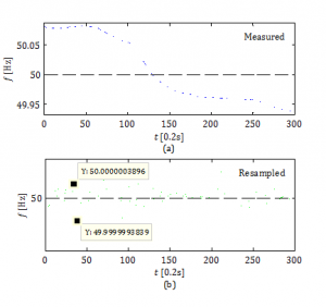
Oversampling of each 10-cycle data blocks before spectrum estimation significantly limits fundamental frequency variation over analysed window and therefore the stationarity assumption is strengthened for frequency component of interest (i.e. linked with the fundamental frequency). As it can be seen in Figure 1 resampling with high precision definitely improves signal quality. The figure presents analysed one minute of acquired voltage waveform and each point is an estimated fundamental frequency over 10-cycle rectangular window. The discrepancy as a difference between two measured values, given in Figure 1(b), is acceptably small and the sample standard deviation is 4.3548•10-6. Please note that scale 0.2s used on abscissa (i.e. horizontal axis) in Figure 1 denotes the step size between neighbouring samples. If there are 300 samples in presented results (as in Figure 1) the total duration is 1 minute (i.e. 0.2s∗300=60s).
It can be seen that both factors such as main tone detection algorithm as well as interpolation algorithm are crucial in appropriate harmonic magnitude and phase estimation. Various interpolation techniques can give different results. The most sophisticated unfortunately are usually the most time consuming. Therefore taking into consideration enormous amount of data to process from few months of multipoint measurements also the interpolation should be optimized and agreement between acceptable accuracy and calculation speed should be found.
Roughly speaking, during interpolation process new samples between existing samples are computed. Different methods were used in data processing such as nearest (coerce) method, linear method, spline method, cubic method, and finite impulse response filter method [1]. The nearest method finds the point nearest to xi in an X array and then assigns the corresponding y value in an interpolated Y to yi. The linear method interpolates yi on the line which connects the two points (xj,xj+1) when the corresponding location xi of interpolated value yi which is located between the two points in an X array. The spline method known also as cubic spline method is almost always the most suitable solution. Within the method the third-order polynomial for each interval between two adjacent points in X (xj,xj+1) is derived. The polynomials have to meet the following conditions: the first and second derivatives at xj and xj+1 are continuous, the polynomials pass all the specified data points, the second derivatives at the beginning and end are zero. The cubic Hermitian spline method is the piecewise cubic Hermitian interpolation. This method is similar to cubic spline interpolation and derives a third-order polynomial but in Hermitian form for each interval (xj,xj+1) and ensures only the first derivatives of the interpolation polynomials are continuous. Compared to the cubic spline method, the cubic Hermitian method is characterized by better local property. The cubic Hermite interpolation method guarantees that the first derivative of the interpolant is continuous and sets the derivative at the endpoints in order to preserve the original shape and monotonicity of the data [2]. Also interpolation based on finite impulse response filter is popular [3], [4]. This method provides excellent results also for frequency analysis, although it is more intensive computationally [2].
| Order | Interpolation method | Computation time [ms] | Marker |
| 1 | Linear | 110 | x |
| 2 | Coerce | 70 | * |
| 3 | Cubic spline | 130 | • |
| 4 | Hermitian spline | 430 | + |
| 5 | FIR filter | 290 | ∗ |
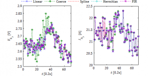
Table above shows the computation time of data interpolation with different algorithms. In each of the cases the presented time is measured for resampling of 10 cycles of measured data. It can be seen that the simplest algorithms exhibit less computation burden. On the other hand in many cases simple algorithms cannot give satisfactory interpolation results and thus affect the harmonic calculation results. Figure 2 shows how different interpolation techniques affect harmonic magnitude estimation from measurements carried out at the LV side of the wind turbine transformer. It can be seen that the coerce method is affected the worst while other algorithms give comparable results.

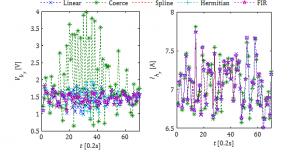
It was observed that in case of more distorted waveforms (e.g. gird-side converter output voltage) interpolation method choice plays a crucial role. In Figure 3 one can see that also linear interpolation and cubic Hermitian spline interpolation do not give satisfactory results. Therefore the most suitable for harmonic components estimation appear to be cubic spline interpolation as well as finite impulse response filter interpolation. Since the spline method (as presented in table above) is less time consuming, this method was used in further data processing. The selected measurement period was selected when the power system frequency were varying below 50 Hz or above 50 Hz.

[1] S. C. Chapra and R. Canale, Numerical Methods for Engineers: With Software and Programming Applications, 6th ed. McGraw-Hill Science, 2009.
[2] National Instruments, "LabVIEW 2011 Help," National Instruments Manual, 2011.
[3] R. A. Losada, "Digital Filters with MATLAB," The Mathworks, 2008.
[4] R. W. Schafer and L. R. Rabiner, "A digital signal processing approach to interpolation," Proceedings of the IEEE, vol. 61, no. 6, pp. 692-702, Jun. 1973.
