Tag: matlab

I was asked few times about possible adjustment of figures in Matlab. Many times there is simply a need to change slightly the default view in order to align with the template in our publication, book, etc. Thus I will try to show few parameters that can easily adjust the view according to our expectations.

Fortunately in Matlab there is an extended flexibility of doing that. I need to admit that it is much more convenient to edit figures in Matlab than in other engineering tools (e.g. LabVIEW, PSCAD, PowerFactory, etc.). Therefore I personally export all of my results into Matlab and later adjust.

Let me explain how to obtain the following figures. As one can see the figures present the same result but slightly in a different way. I do not need to mention that nicely presented research results can easily attract broader audience. Hence even in the conservative scientific world it is of great importance to be able selling our findings.

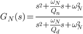
The figures above show the variation of notch filter depending on the quality factor. The filter is tuned for 100Hz and included in synchronous reference frame and afterwards represented in natural/stationary reference frame. Thus the resonant peaks are shifted ±50Hz. The notch filter transfer function is expressed in the following way.

Such figures can be obtained by using the following code. Please note that also Control System Toolbox is needed to obtain the frequency response of the notch filter.

% Prepare workspace
clc, clear('all'), close('all'),
% Define font parameters
fontname= 'Cambria';
set(0,'defaultaxesfontname',fontname);
set(0,'defaulttextfontname',fontname);
fontsize= 10;
set(0,'defaultaxesfontsize',fontsize);
set(0,'defaulttextfontsize',fontsize);
% Get screen resolution
scrsz= get(0,'ScreenSize');

%% Notch filter
% Define frequency parameters
f= 50;                    % Grid frequency [Hz]
omegaO= 2*pi*f;           % Angular frequency [rad/s]
omegaN= 2*omegaO;         % Resonant frequency [rad/s]
step= 0.1;                % Frequency step [Hz]
frequencySeries= 1:step:200;
omegaSeries= 2*pi*frequencySeries;
% Construct transfer function
s= tf('s');
sN= s-1i*omegaO;
sP= s+1i*omegaO;
% Allocate memory
firstIndex= 1; lastIndex= 30; k= 1;
surfTf= zeros(length(frequencySeries),lastIndex);
map= zeros(lastIndex,3);

%% Display results
% Initiate figure
f1= figure('Name','Transfer Function Plot',...
'Position',[scrsz(3)*0.2 scrsz(4)*0.2 scrsz(3)*0.35 scrsz(4)*0.45]);
hold('on'),
for index=firstIndex:k:lastIndex,
     Qn= 100/sqrt(2); Qd= index+5;           % Quality factor
     GnN= (sN^2+omegaN*sN/Qn+omegaN^2)/(sN^2+omegaN*sN/Qd+omegaN^2);
     GnP= (sP^2+omegaN*sP/Qn+omegaN^2)/(sP^2+omegaN*sP/Qd+omegaN^2);
     Gn= 1/2*(GnP+GnN);                      % From SRF to NRF
     [magGn,phaseGn]= bode(Gn,omegaSeries);  % Frequency response
     GnCplx= magGn.*exp(1i*phaseGn);
     surfTf(:,index)= GnCplx(:);
     sub1= subplot(2,1,1,'Parent',f1);box(sub1,'on'),hold(sub1,'all'),
     plot(frequencySeries,abs(GnCplx(:)),...
          'Color',[0 1-index/lastIndex index/lastIndex]),
          ylabel('|{\itG_{notch}}| [abs]'),
          xlim([min(frequencySeries) max(frequencySeries)]),
          ylim([0.5 1.02]),hold('on'),grid('off'),
     sub2= subplot(2,1,2,'Parent',f1);box(sub2,'on'),hold(sub2,'all'),
     plot(frequencySeries,180*unwrap(angle(GnCplx(:)))/pi,...
          'Color',[0 1-index/lastIndex index/lastIndex]),
          xlim([min(frequencySeries) max(frequencySeries)]),
          ylim([-1100 1300]),hold('on'),grid('off'),
          ylabel('\angle{\it{G_{notch}}} [\circ]'),xlabel('{\itf} [Hz]'),
     map(index,:)= [0 1-index/lastIndex index/lastIndex];
end
c1= colorbar('peer',sub1,'East');colormap(map),
set(c1,'YTickMode','manual','YTickLabelMode','manual',...
 'YTick',[firstIndex; floor((lastIndex-firstIndex)/2); lastIndex],...
 'YTickLabel',[firstIndex+5; floor((lastIndex-firstIndex)/2)+5; lastIndex+5]),
hold('off'),

f2= figure('Name','Impedance Angle',...
     'Position',[scrsz(3)*0.2 scrsz(4)*0.2 scrsz(3)*0.35 scrsz(4)*0.45]);
ax2= axes('Parent',f2);grid(ax2,'on'),hold(ax2,'all'),
mesh(180*unwrap(angle(surfTf))/pi),zlabel('\angle{\it{G_{notch}}} [\circ]'),
     ylabel('{\itf} [Hz]'),xlabel('{\itQ_n} ','Rotation',322),view([60 40]),
set(gca,'XTick',[firstIndex; floor((lastIndex-firstIndex)/2); lastIndex],...
 'XTickLabel',[firstIndex+5; floor((lastIndex-firstIndex)/2)+5; lastIndex+5],...
 'YTick',1:50/step:length(frequencySeries),...
 'YTickLabel',min(frequencySeries):50:max(frequencySeries)),

Feel free to use and modify included Matlab code. I am also looking forward to hear from you in case of any suggestions and comments.

References

[1] Ł. Kocewiak, Ch. Buchhagen, R. Blasco-gimenez, J. B. Kwon, M. Larsson, Y. Sun, X. Wang et al., “Multi-frequency stability of converter-based modern power systems,” Technical Brochure 928, Page(s) 1-147, CIGRE, March 2024.
[2] Ł. Kocewiak, R. Blasco-Gimenez, C. Buchhagen, J. B. Kwon, M. Larsson, Y. Sun, X. Wang, “Practical Aspects of Small-signal Stability Analysis and Instability Mitigation,” in Proc. The 21st Wind & Solar Integration Workshop, 12-14 October 2022, The Hauge, The Netherlands.
Categories
Software
How to adjust figures in Matlab?