Categories
Product Management Software

The 6 Phases of Product Lifecycle: Idea, Explore, Validate, Grow, Sustain, Retire

Product Lifecycle Management (PLM) describes how a product evolves from an initial idea to eventual retirement. The lifecycle helps organizations manage uncertainty in early stages while focusing on growth and profitability once a product proves its market fit. Each of 6 phases has a different purpose, timeframe, and success metrics. Early stages (i.e. Idea, Explore, Validate) emphasize learning and experimentation with potential customers, while later stages (e.g. Grow, Sustain, Retire) focus on scaling, operational efficiency, and financial performance. Understanding these phases helps allocate people effectively and manage products throughout their entire lifecycle.
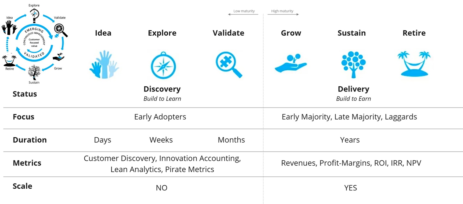
Phases of Product Lifecycle

Idea

The Idea phase is where potential product opportunities are identified. Teams recognize customer problems, unmet needs, or market gaps that could lead to valuable solutions. Ideas may come from customer feedback, technological advances, internal innovation, or strategic business goals. At this stage, concepts are still rough hypotheses rather than defined products. The goal is to quickly assess whether the opportunity is worth exploring further. Activities typically include problem framing, initial discussions, and collecting early insights from users or the market.

Explore

The Explore phase focuses on understanding the problem space and identifying possible solution approaches. Teams conduct research to learn about user needs, behaviors, and market conditions. The objective is to confirm that the problem is real and significant. Activities may include user interviews, market analysis, early concept sketches, and exploratory prototypes. Multiple ideas can be evaluated during this phase. The emphasis is on learning and reducing uncertainty before committing significant development effort.

Validate

The Validate phase tests whether the proposed solution effectively solves the identified problem and creates value for users. Teams develop prototypes or minimum viable products (MVPs) and test them with early adopters. Experiments and usability testing help verify assumptions about desirability, usability, and feasibility. Metrics such as user engagement, activation, and retention are often monitored. The aim is to confirm product–market fit and ensure that the solution is viable before scaling development and investing in broader delivery.

Grow

The Grow phase begins once the product has demonstrated clear value and product–market fit. The focus shifts to increasing adoption and expanding the customer base. Teams improve reliability, performance, and user experience while adding features that strengthen the product’s value proposition. Marketing and distribution efforts intensify to reach a wider audience. Infrastructure and support capabilities are also scaled to accommodate growth. Key indicators during this phase include adoption rates, revenue growth, and customer retention.

Sustain

The Sustain phase represents the maturity of the product. Adoption has stabilized and the product delivers consistent value to customers and the business. Development efforts emphasize incremental improvements, reliability, and operational efficiency rather than major innovation. Teams focus on maintaining competitiveness through updates, performance improvements, and cost optimization. Financial indicators such as profitability, margins, and operational efficiency become important measures of success as the product continues serving established customer segments.

Retire

The Retire phase marks the end of the product lifecycle when the product is gradually phased out or replaced. This may occur due to declining demand, technological change, or the introduction of more advanced solutions. The main objective is to manage the transition responsibly while minimizing disruption for users. Organizations typically communicate end-of-life plans, support migration to newer products, and maintain limited support during the transition period before fully discontinuing development and service.

In short

The product lifecycle describes how a product evolves from an initial idea to its eventual retirement. It begins with identifying opportunities and exploring potential solutions, followed by validating whether the product delivers real value to users. Once proven, the focus shifts to scaling adoption and growing the product in the market. As the product matures, efforts concentrate on sustaining performance and maximizing long-term value. Finally, when the product becomes outdated or demand declines, it is gradually retired while customers transition to newer solutions.

PhasePurposeKey ActivitiesPrimary FocusTypical Metrics
IdeaIdentify potential opportunities and problems worth solvingOpportunity identification, problem framing, initial discussions, gathering insightsRecognizing customer needs and market gapsNumber of ideas, problem relevance, strategic alignment
ExploreUnderstand the problem space and possible solutionsUser research, market analysis, concept sketches, exploratory prototypesLearning about users and evaluating solution optionsResearch insights, validated problem statements, concept feasibility
ValidateTest whether the proposed solution delivers real valueMVP development, experiments, usability testing, early user feedbackConfirming product–market fit and solution viabilityUser engagement, activation, retention, experiment results
GrowScale adoption and expand market presenceFeature development, infrastructure scaling, marketing, performance improvementsIncreasing customer base and market penetrationAdoption rate, revenue growth, customer acquisition, retention
SustainMaintain value and optimize product performanceIncremental improvements, maintenance updates, cost optimizationStability, efficiency, and profitabilityProfit margins, operational efficiency, customer satisfaction
RetirePhase out the product and transition usersEnd-of-life planning, communication, migration support, service shutdownResponsible product discontinuationRemaining user base, migration rate, support cost reduction

References

[1] Theodore Levitt, “Exploit the Product Life Cycle,” Harvard Business Review, 1965.
[2] Philip Kotler, Kevin Lane Keller, “Marketing Management,” Pearson, 2021.
[3] Steve Blank, Bob Dorf, “The Startup Owner's Manual – The Step-By-Step Guide for Building a Great Company,” John Wiley & Sons, 2020.
[4] Tendayi Viki, “The Lean Product Lifecycle,” Medium, 30 November 2018.

Categories
Software

How to adjust figures in Matlab?

I was asked few times about possible adjustment of figures in Matlab. Many times there is simply a need to change slightly the default view in order to align with the template in our publication, book, etc. Thus I will try to show few parameters that can easily adjust the view according to our expectations.

Fortunately in Matlab there is an extended flexibility of doing that. I need to admit that it is much more convenient to edit figures in Matlab than in other engineering tools (e.g. LabVIEW, PSCAD, PowerFactory, etc.). Therefore I personally export all of my results into Matlab and later adjust.

Let me explain how to obtain the following figures. As one can see the figures present the same result but slightly in a different way. I do not need to mention that nicely presented research results can easily attract broader audience. Hence even in the conservative scientific world it is of great importance to be able selling our findings.

Notch Filter - Bode Plot
Notch Filter - 3D Phase

The figures above show the variation of notch filter depending on the quality factor. The filter is tuned for 100Hz and included in synchronous reference frame and afterwards represented in natural/stationary reference frame. Thus the resonant peaks are shifted ±50Hz. The notch filter transfer function is expressed in the following way.

Such figures can be obtained by using the following code. Please note that also Control System Toolbox is needed to obtain the frequency response of the notch filter.

% Prepare workspace
clc, clear('all'), close('all'),
% Define font parameters
fontname= 'Cambria';
set(0,'defaultaxesfontname',fontname);
set(0,'defaulttextfontname',fontname);
fontsize= 10;
set(0,'defaultaxesfontsize',fontsize);
set(0,'defaulttextfontsize',fontsize);
% Get screen resolution
scrsz= get(0,'ScreenSize');

%% Notch filter
% Define frequency parameters
f= 50;                    % Grid frequency [Hz]
omegaO= 2*pi*f;           % Angular frequency [rad/s]
omegaN= 2*omegaO;         % Resonant frequency [rad/s]
step= 0.1;                % Frequency step [Hz]
frequencySeries= 1:step:200;
omegaSeries= 2*pi*frequencySeries;
% Construct transfer function
s= tf('s');
sN= s-1i*omegaO;
sP= s+1i*omegaO;
% Allocate memory
firstIndex= 1; lastIndex= 30; k= 1;
surfTf= zeros(length(frequencySeries),lastIndex);
map= zeros(lastIndex,3);

%% Display results
% Initiate figure
f1= figure('Name','Transfer Function Plot',...
'Position',[scrsz(3)*0.2 scrsz(4)*0.2 scrsz(3)*0.35 scrsz(4)*0.45]);
hold('on'),
for index=firstIndex:k:lastIndex,
     Qn= 100/sqrt(2); Qd= index+5;           % Quality factor
     GnN= (sN^2+omegaN*sN/Qn+omegaN^2)/(sN^2+omegaN*sN/Qd+omegaN^2);
     GnP= (sP^2+omegaN*sP/Qn+omegaN^2)/(sP^2+omegaN*sP/Qd+omegaN^2);
     Gn= 1/2*(GnP+GnN);                      % From SRF to NRF
     [magGn,phaseGn]= bode(Gn,omegaSeries);  % Frequency response
     GnCplx= magGn.*exp(1i*phaseGn);
     surfTf(:,index)= GnCplx(:);
     sub1= subplot(2,1,1,'Parent',f1);box(sub1,'on'),hold(sub1,'all'),
     plot(frequencySeries,abs(GnCplx(:)),...
          'Color',[0 1-index/lastIndex index/lastIndex]),
          ylabel('|{\itG_{notch}}| [abs]'),
          xlim([min(frequencySeries) max(frequencySeries)]),
          ylim([0.5 1.02]),hold('on'),grid('off'),
     sub2= subplot(2,1,2,'Parent',f1);box(sub2,'on'),hold(sub2,'all'),
     plot(frequencySeries,180*unwrap(angle(GnCplx(:)))/pi,...
          'Color',[0 1-index/lastIndex index/lastIndex]),
          xlim([min(frequencySeries) max(frequencySeries)]),
          ylim([-1100 1300]),hold('on'),grid('off'),
          ylabel('\angle{\it{G_{notch}}} [\circ]'),xlabel('{\itf} [Hz]'),
     map(index,:)= [0 1-index/lastIndex index/lastIndex];
end
c1= colorbar('peer',sub1,'East');colormap(map),
set(c1,'YTickMode','manual','YTickLabelMode','manual',...
 'YTick',[firstIndex; floor((lastIndex-firstIndex)/2); lastIndex],...
 'YTickLabel',[firstIndex+5; floor((lastIndex-firstIndex)/2)+5; lastIndex+5]),
hold('off'),

f2= figure('Name','Impedance Angle',...
     'Position',[scrsz(3)*0.2 scrsz(4)*0.2 scrsz(3)*0.35 scrsz(4)*0.45]);
ax2= axes('Parent',f2);grid(ax2,'on'),hold(ax2,'all'),
mesh(180*unwrap(angle(surfTf))/pi),zlabel('\angle{\it{G_{notch}}} [\circ]'),
     ylabel('{\itf} [Hz]'),xlabel('{\itQ_n} ','Rotation',322),view([60 40]),
set(gca,'XTick',[firstIndex; floor((lastIndex-firstIndex)/2); lastIndex],...
 'XTickLabel',[firstIndex+5; floor((lastIndex-firstIndex)/2)+5; lastIndex+5],...
 'YTick',1:50/step:length(frequencySeries),...
 'YTickLabel',min(frequencySeries):50:max(frequencySeries)),

Feel free to use and modify included Matlab code. I am also looking forward to hear from you in case of any suggestions and comments.

Categories
Software

Change font name in Bode plot

I had been struggling with this problem a while before I did manage to find a work around. It was actually quite important for me to change the font name in Bode plots because I decided to use everywhere Cambria in my report. Normally Heveltiva is used by default in Matlab.

In general it is possible to change font in Matlab plots without any problems. But this is in case the standard package. It should be emphasized that each of Matlab toolboxes is developed by separated teams of specialists. That is why sometimes different features can be solved with a different approach and actually in Control System Toolbox it is not predicted to change font name. You can change the size or style but not the name.

Available parameters for different labels in case of Bode, Nyquist, etc. plots are the following

>> PlotHandle= bodeplot(TrunsferFunction);
>> PlotOptions= getoptions(PlotHandler);
>> PlotOptions.Title,
ans =

String: 'Dummy Title'
FontSize: 10
FontWeight: 'normal'
FontAngle: 'normal'
Color: [0 0 0]
Interpreter: 'tex'

As everyone can see there is not option defining the font name. Fortunately there is some space to deal with it due to the fact that it is possible to define the interpreter. In Tex it is actually possible to define font name locally in text. This can be done in the following way

PlotOptions.Title.String= '';
PlotOptions.XLabel.String= '\fontname{Cambria}{\itf}';
PlotOptions.XLabel.FontSize= 10;
PlotOptions.YLabel.String= {'\fontname{Cambria}|{\itG_{ol}}|',...
    '\fontname{Cambria}\angle{\itG_{ol}}'};
PlotOptions.YLabel.FontSize= 10;
PlotHandle.setoptions(PlotOptions),

And here is the final result.

Bode Plot Font NameAnother solution is to get the frequency response into arrays and display results using functions form Matlab base package. In this case it is also possible to change axes font name.

You can also change the default system font for all figures and axes by putting the following code at the beginning of your m-file. Please note that this will change your default font during your Matlab session. I do this quite often if I do not want to think so much preparing figures for printing.

fontname= 'Cambria';
set(0,'defaultaxesfontname',fontname);
set(0,'defaulttextfontname',fontname);
fontsize= 10;
set(0,'defaultaxesfontsize',fontsize);
set(0,'defaulttextfontsize',fontsize);

Hope this helps and looking forward to see some comments.

Categories
Software

Shapes in deep shadows and high lights in Matlab

Normally I work in different toolboxes of Matlab on purpose. Either it is for my research project purposes  or due to my research project purposes. That is why I came up with an idea to do something in Matlab that would not have any application. I wanted to do something what would look nice and be by itself. Later of course I found some interesting application areas of my work but let us start from the beginning.

Łukasz Kocewiak
Photograph by Magdalena Sozańska

I decided to use Image Processing Toolbox because, in my opinion, no matter of what working on images should always give interesting results. Why not to use some of my pictures from the past taken with my old Minolta Dynax 700si. I still should have it somewhere in the basement.

%% Gausian convolution matrix
G= [1  4  7  4 1;
    4 16 26 16 4;
    7 26 41 26 7;
    4 16 26 16 4;
    1  4  7  4 1];
G= G/sum(sum(G));

%% Picture analysis
ExampleUint= imread('Example.jpg');
ExampleDouble= double(ExampleUint);
[m n]= size(ExampleDouble(:,:,1));

%%  Linear Gaussian filter
ExampleFilterUint= imfilter(ExampleUint,G,'conv');
for k=1:10,
    ExampleFilterUint= imfilter(ExampleFilterUint,G,'conv');
    k= k+1; %#ok<FXSET>
end
ExampleFilterDouble= double(ExampleFilterUint);

Due to the fact that the picture was taken still in analog technology and scanned in any photo lat the quality is not so good. Even in the small picture (a) noise can be clearly seen. I decided to get rig of it by application of a digital filter. A lot of noise and sharp edges that can affect the final result. In order to make the picture more smooth we will use a low-pass filter (b). I decided to use Gaussian filter with the convolution matrix as presented above.

Łukasz Kocewiak 3DThis apprioach can be succesfully used if we would like to evaluate how objects are shaped by light. A good example is in case of body shaping by either attending gym or fitness. If we simply cannot assess if our muscles are sufficiently shaped, just take a picture and do some processing in Matlab. Probably other applications can be found. Please let me know if you have any suggestions by posting a comment.

And an exemplary code from Matlab showing how to display two-dimensional matrix of double precision numbers.

scrsz= get(0,'ScreenSize');
%% Show results
fi1= figure('Name','3D Plot',...
     'Position',[0.1*scrsz(3) 0.1*scrsz(4) 0.35*scrsz(3) 0.5*scrsz(4)]);
ax1= axes('Parent',fi1,'FontName','Verdana','FontSize',10);
grid(ax1,'on'),hold(ax1,'all'),
mesh(ExampleFilterDouble(:,:,1)),colormap('hot'),
view(ax1,[-150 70]),xlim([0 n]),ylim([0 m]),
Categories
Software

How to open SVG 1.1 in Visio 2007

A while ago I had a horrible problem with MS Visio 2007. I was really happy that I did manage to prepare nice vector graphics in Adobe Illustrator CS4. Among others it was a map indicating one of onshore wind farms that I analyze within the confines of my research project. Normally at work I do not have such fancy tools as Adobe software, so I had to save results in something that MS Visio would be able to open.

Clipping Path 1
Vector graphics created in Adobe Illustrator CS4.


I decided to use an open standard vector format such as SVG is. Since it is an open standard it should be possible to easily save it in Illustrator and hypothetically without any problems open in Visio. I would like to emphasize that this version (i.e. SVG 1.1)  was developed in 2003 as it is stated on the W3C website. Actually Visio can deal with SVG 1.1 but in a selective manner. How big was my disappointment when I realized that actually well described in the standard clipping path is not supported.

The same drawing with visible clipping path.

The description of the clipping path (commonly known in popular vector graphics applications) can be found on the W3C (Clipping Path) website. An exemplary code showing an application of the clipping path from an SVG file generated by Adobe Illustrator looks in the following way

<defs>
     <path id="SVGID_1_" d="M111.478,271.964c0,0-5.669,0-5.669,5.478z"/>
</defs>
<clipPath id="SVGID_2_">
     <use xlink:href="#SVGID_1_"  overflow="visible"/>
</clipPath>

If one would like to open such kind of SVG file with clipping path in Visio the error dialog box appears which is presented below. MS Visio 2007 is simply not capable to open files  including clipping path definitions. I tried to find any solution how to deal with this problem via Internet but unsuccessfully.

In the error log file generated by the software it is clearly stated which elements from SVG structure are incompatible. One of possibilities to work around this problem is to delete unsupported fragments of the code. Of course this would affect that elements of our vector graphics which should be hidden by the clipping path will be visible.

[Warning] DataType: Element <clipPath>
Context: Line 13 ID SVGID_2_
Description: Invalid children of clip-path element. Children removed

Please remember also to remove information about the clipping path from each of elements included in the vector graphics. Later in MS Visio 2007 it is possible to use other methods of masking unwanted elements or parts of them.

I hope this help and please shear your experience with me regarding this problem by adding a comment. Cheers!